GXquery 4.0 Lab - Exercise 5

This documentation is valid for:

This is part of the GXquery 4.0 Lab and should be done after Exercise 4.

The purpose of this exercise is to show how conditional styles are created.

What are the conditional styles?

Highlighting values according certain conditions is often more eye-catching.

For example, in this exercise we will create a Pivot table in which to show the amounts of money of sales for each airline by country and city. The Sales Analyst in charge of analyzing the Travel Agency sales has requested us to highlight with color the amounts according to the following criteria:

1. Highlight sales under 1000 with red.
2. Highlight sales between 1000 and 9999 with blue.
3. Highlight sales over 9999 with green.

Next, we will see how to do this.

Step 1

1. Create the following Pivot table as you can see in Exercise 1. Name it as you wish or leave the name proposed by GXquery:

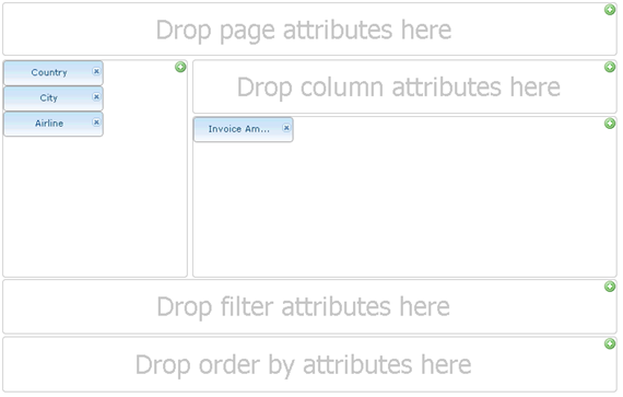
2. Select the List tab on the Attributes panel.

3. Use the Filter cell in the Attributes window to quickly find the attributes shown in the image. These are:

Country → drag it into the “Drop row attributes here” sector
City → drag it into the “Drop row attributes here” sector
Airline → drag it into the “Drop row attributes here” sector
Invoice Amount → drag it into the “Drop data attributes here” sector to obtain totals per file.

Step 2

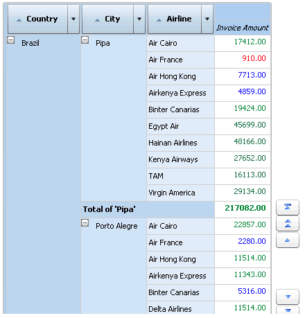
Press View. You should see an image similar to the one below.

Step 3

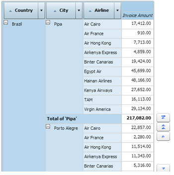
Press Edit to return to the table editing status. Click on the Invoice Amount element; it will appear with its properties on the Properties:Query Element panel (bottom right).

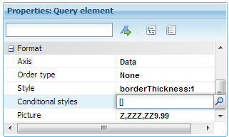
Note that there is an expandable property named Format. Click on the node to open it.

On the Format list, find the Conditional styles property and click on the “[]” value it contains, and a small magnifier will appear on the right, as shown below.

Step 4

Click on the magnifier. The following dialogue window will appear.

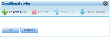
In order to apply conditional styles, we must tell GXquery what we want to restrict, and this is done through Rules. A rule is an instruction of the «If this happens, then do that» type.

Now click on the Insert rule image. You will see the following image.

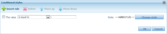
This is a wizard that will help you build the rules. Then, to the right of the first combo box, whose value “is less than”, enter the value 1000.

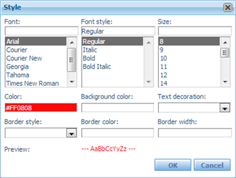
Now click on the Change style button to open the Style dialogue box, go to the Color cell and select red. Then press OK. With this, we have set the first rule: “Highlight sales under 1000 with red”.

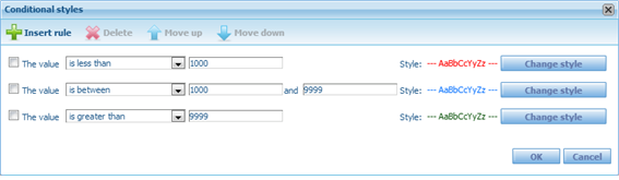
Select the magnifier of the Conditional styles property once again to define the second rule, where values between 1000 and 9999 must be highlighted in blue. To do so, we will select the “is between” value from the combo. You will see that a new cell is added to the right to narrow the range. Next, write 1000 on the first line of the cell, and 9999 on the second. Then select the color blue, as you previously did.

For the third rule, select the “is greater than” value from the combo, write 9999 to the right, and assign the color green.

The dialogue should look like the following image. Finally, press OK to return to the editing window.